Image Formation Concepts

pyBSM replicates image formation based on the physical and electronic characteristics of the sensor and scene. The pyBSM image formation chain consists of 4 separate components:

• 3D World: Physical geometry and materials of the scene

• Atmosphere: Scattering, absorption, and turbulence

• Optics: Image formation through lenses and apertures

• Sensor and Electronics: Detection, digitization, and noise modeling

These components are illustrated below:

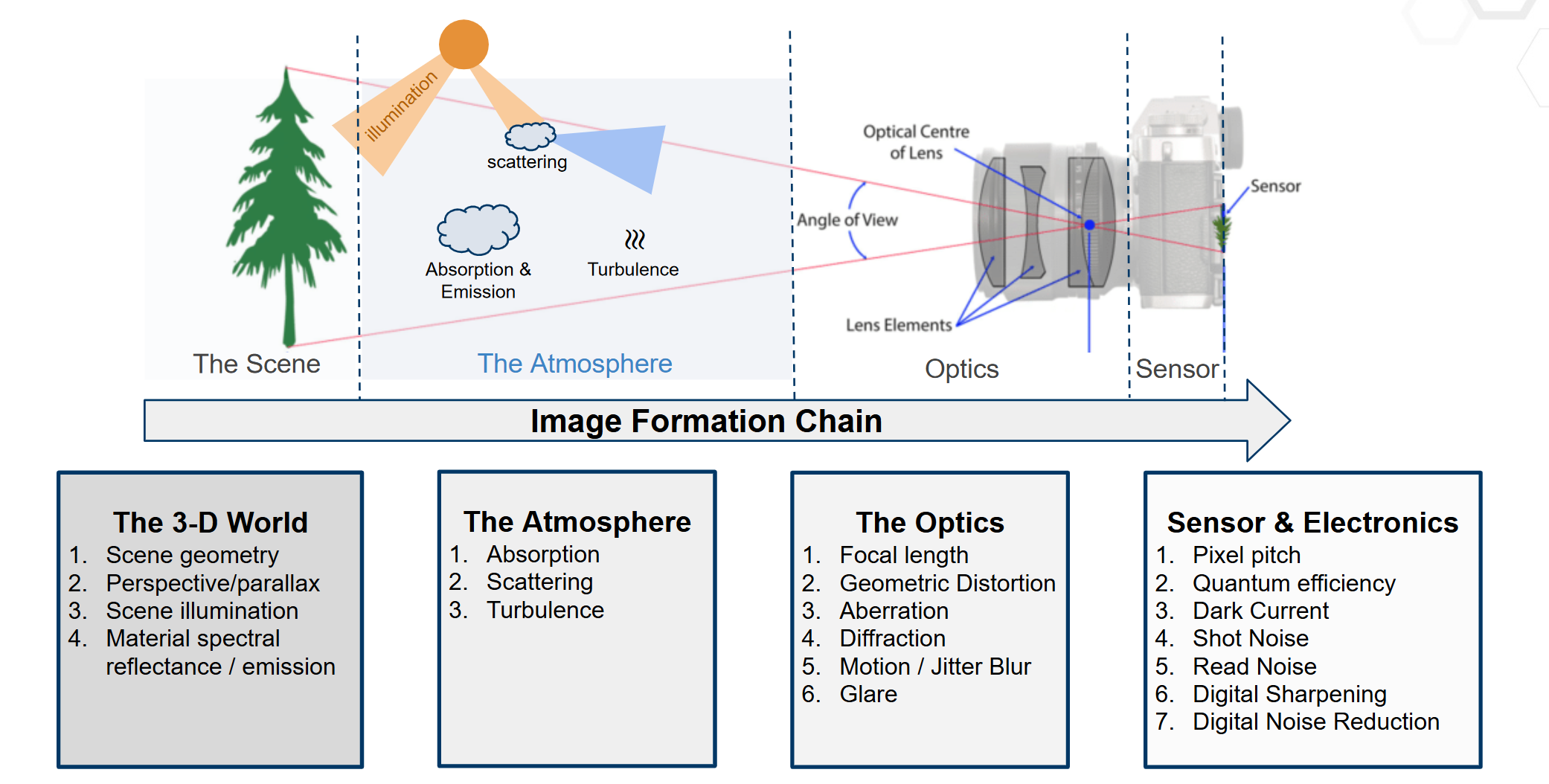
Figure 1: This modular structure underpins all simulations in pyBSM.

Ultimately, pyBSM bases its models and simulations around this image formation pipeline.

Point-Spread Function (PSF) and Optical Transfer Function (OTF)

pyBSM is built on the principle of translation-invariant systems, or that the image process can be described by a set of functions that degrade the ideal image scenario. Fundamental to this principle is the simulation of Point-Spread Functions (PSFs) and Optical Transfer Functions (OTFs), which describe how an ideal scene is transformed as light reaches the sensor. A PSF is a function that is convoluted with the scene to create the degradations, while at OTF is the same thing except in the frequency domain (i.e. an OTF is the Fourier transform of a PSF). An OTF which has large values for certain frequencies will faithfully replicate those frequencies on the sensor, while low values would diminish or remove those frequencies entirely. For example, a diffraction-based OTF would have low values for frequencies above Abbe’s diffraction limit, since the lens cannot reconstruct these frequencies. This OTF would also therefore change based on the optics used, as a larger numerical aperture would afford a larger Abbe’s diffraction limit. A perfect and ideal OTF would be equal to 1 for all frequency values.

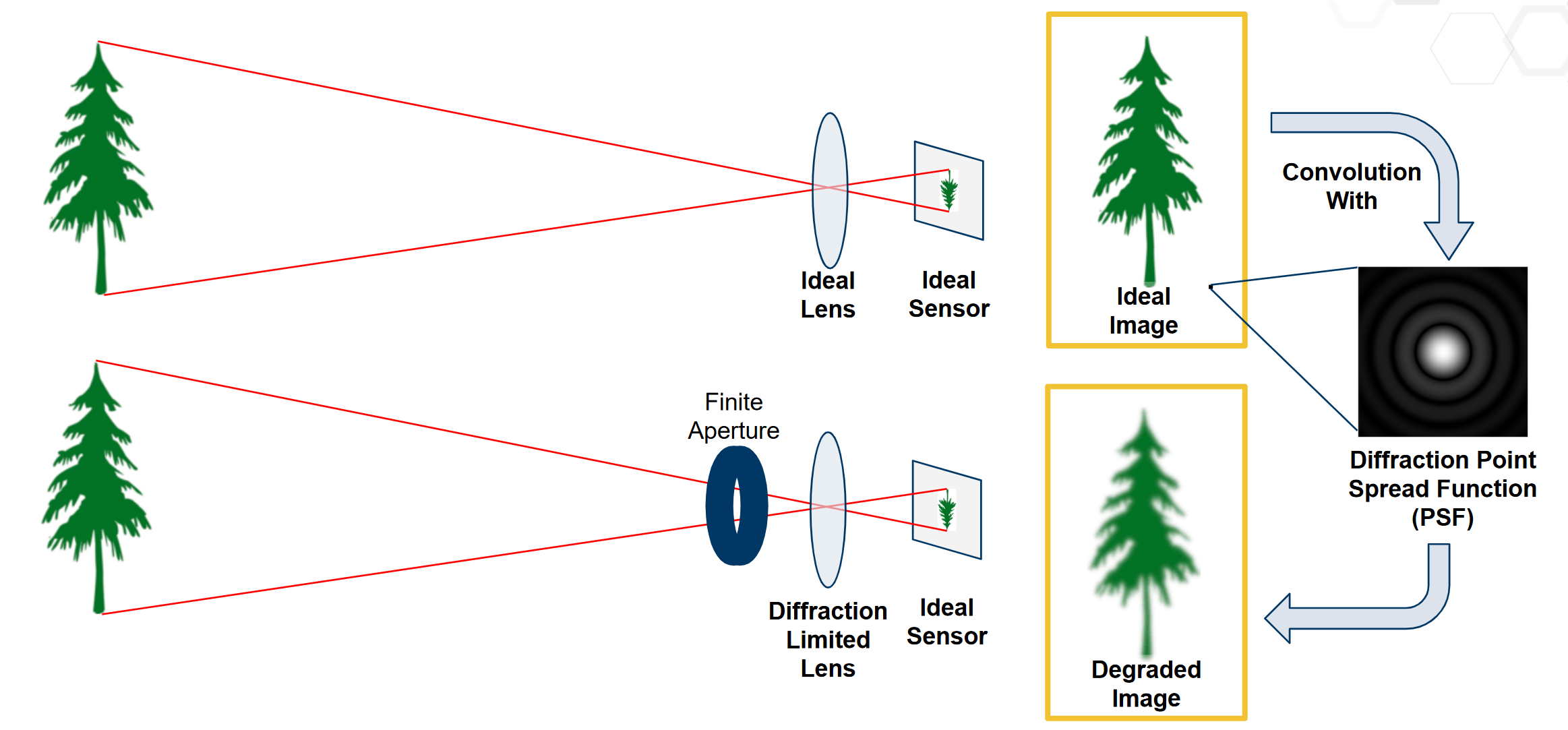
Figure 2: Description of PSFs

In pyBSM, the overall OTF and PSF of the system is called the “Composite System PSF”, and is composed of a combination of the PSFs from all the separate components:

• Turbulence

• Jitter and Drift

• Diffraction

• Defocus

• Wavefront

• Charge Diffusion

• Detector

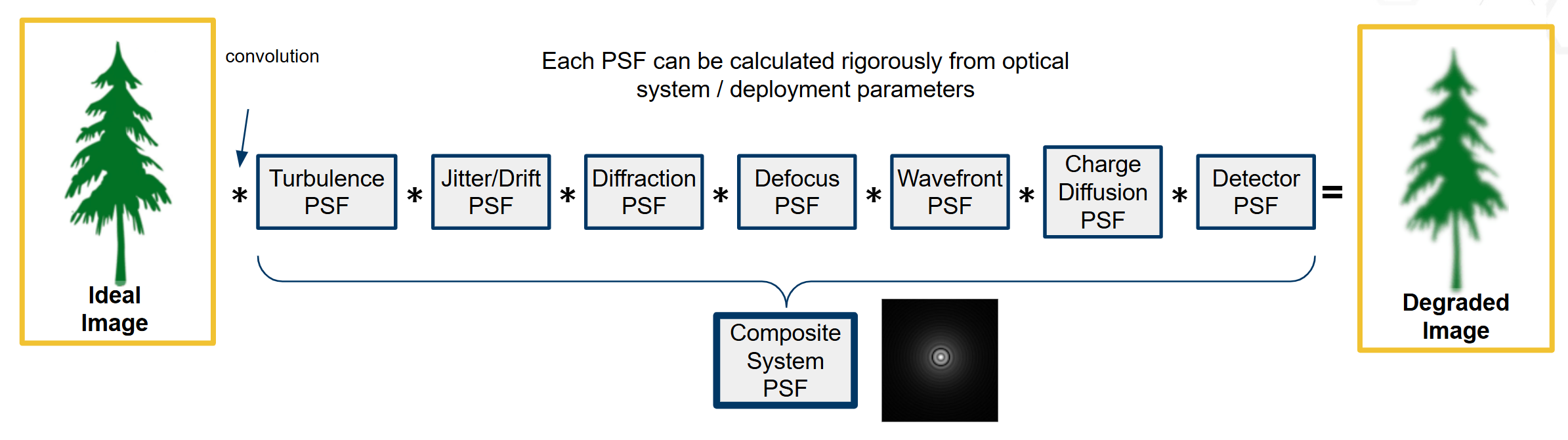
Figure 3: Depiction of all PSFs in pyBSM

It is important to note that each PSF degrades the ideal image and cannot enhance resolution. However, the interplay and combination of many PSFs together is complex. Some examples of these OTFs are in NRTK/docs/examples/otf_visualization.ipynb

Image Simulation

pyBSM allows the user to simulate different environmental or sensor effects for a given reference image and therefore simulate new OTFs. Some practical examples include if the user wants to increase the sensor noise, change the distance from the sensor to target, increase environmental wind speed, or change the aperature size of the lens.

To simulate the effects of these variables, pyBSM simulators are composed of three elementary classes:

• Sensor: Defines the physical and electronic characteristics of the sensor and optics, including pixel pitch, focal length, aperture diameter, sensor noise, and spectral response.

• Scenario: Captures details about the environment and scene, such as the observer’s altitude and speed, atmospheric conditions, and the reflectance and temperature of the target.

• Reference Image: Represents the baseline or ideal image from which degradations are simulated. It includes pixel intensity values, ground sampling distance (GSD), and optionally a mapping between pixel values and reflectance.

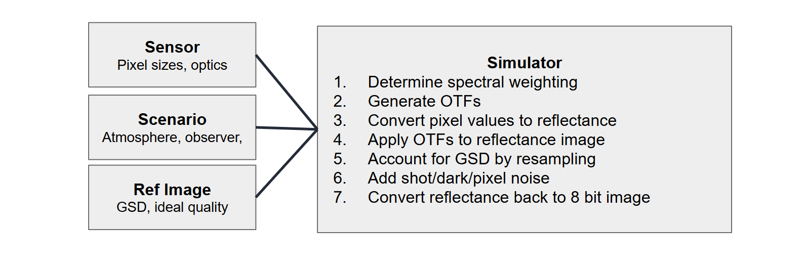
Figure 4: Depiction of simulator pipeline

An example notebook simulation is included in NRTK/docs/examples/pybsm/pybsm_test.ipynb

Main Sensor Variables

The sensor class has the most variables in the simulator. If these are unknown or unspecified, they can be estimated via the “estimate_capture_parameters” function in the ref_image class, but oftentimes they can be determined by the camera’s datasheet.

Overall, the main variables of interest can be separated into several categories:

Pixel Size Parameters: These include changes in the image due to the geometrical pixel sizes

• p_x, p_y: center-to-center spacing between pixels in the x/y directions (meters). This is also known as pixel_pitch, and this will change the resolution of the resulting image. Note if p_y is not provided, it is assumed to be equal p_x`` (p_x is required, p_y can be None).

• w_x, w_y: actual width of the photoreceptive component of the pixel (meters). Note that this should always be less than p_x , p_y, since this describes the “fill factor.”” If w_x = p_x and w_y = p_y, fill factor is 1 and the entire pixel is photoreceptive. If w_x = 1/2 * p_x and w_y = 1/2 * p_y, then the fill factor is .25 since the photoreceptive component only comprises 25% of the entire sensor area (default None).

Lens and Optics These parameters determine the projection of the scene onto the sensor:

• f: focal length of the lens (meters). A large focal length typically has a narrower field-of-view with compressed depth of the scene, while a smaller focal length has a wider field-of-view with exaggerated and distorted perspectives (required).

• D: effective aperture diameter of the lens (meters). This is related to the f-number (f#) of the lens, which defines the how much light is reaching the sensor alongside the depth of field and diffraction. A small aperture (i.e. small f#) results in less light and shallower depth-of-field but less diffraction and sharper images, while a large aperture (i.e. large f#) results in more light and deeper depth-of-field but less sharp images (required).

Here is a depiction of the pixel size and optics variables:

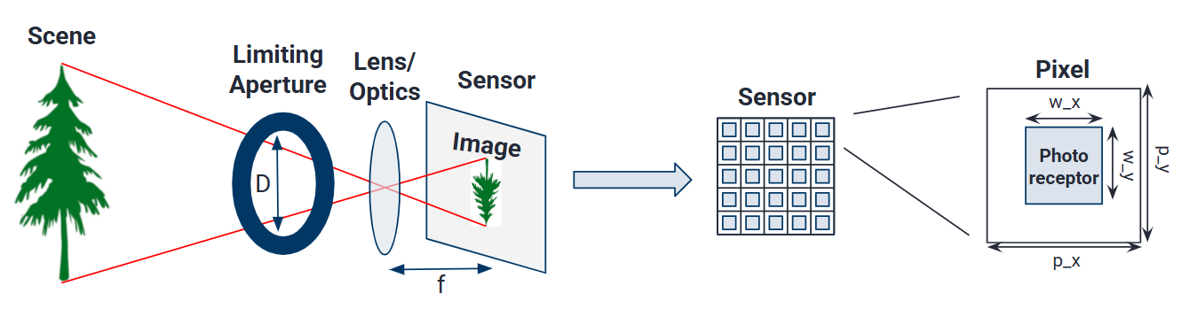
Figure 5: Depiction of sensor variables

Spectral Response These parameters define how the sensor responds to different wavelengths of light:

• qewavelengths, qe: the detector quantum efficiency (QE) of the corresponding wavelengths (microns). QE defines what percentage of the incoming photons are converted to electrons by the sensor, where sensor which has a large QE with respect to a specific wavelength will capture that color more strongly than it would to one with a smaller QE. Note that QE cannot be greater than 1, as 1 is perfect efficiency. Most sensors will have the QE published. For a generic, high quality back-illuminated (BI) silicon sensor the values would be: qewavelengths: [0.3, 0.4, 0.5, 0.6, 0.7, 0.8, 0.9, 1.0, 1.1] (default is opt_trans_wavelengths)

• qe: [0.05, 0.6, 0.75, 0.85, 0.85, 0.75, 0.5, 0.2, 0] (default ones).

• opt_trans_wavelengths: specifies the start and end wavelengths the camera captures (meters). This is the “spectral bandpass.”” Unless the optics of the camera are set specifically to isolate certain colors, this can be set as wide as the quantum efficiency, so the previous example would be 0.3e-6 to 1.1e-6 (required).

Noise and Signal Quality: These capture the noise and signal-to-noise (SNR) characteristics of the camera.

• int_time: maximum integration time of the sensor, or how long it converts photons to electrons (seconds). Also known as “exposure time.” We use the term “maximum” since the image will be clipped depending on the monitor well fill percentage (i.e. max_n) (default 1.0).

• bit_depth: How many bits are used to represent the values in each pixel (bits). Standard 0-255 images are 8-bit, while larger bits capture more signal and a larger dynamic range of values (default 100.0).

• read_noise: electron noise created in reading out the pixels (root-mean squared electrons). This is especially problematic in dark scenes where the captured signal is low in which the read noise can overwhelm it (default 0.0).

• dark_current: the small amount of electrons going through each pixel even when no photons are entering (electrons per second). Dark current is what typically overwhelms low-light images (default 0.0).

• max_n: the detector electron well capacity (electrons). This is the maximum amount of electrons that can be captured by each pixel in the integration time (default is 100e6).

• optics_transmission: full system, in-band optical transmission (unitless). Not counting other qualities, how much of received light is captured by camera where the minimum is 0 and maximum is 1 (default ones).

• s_x, s_y: root-mean-squared jitter amplitudes in the x and y directions (radians). These correspond to small, rapid motions that could come from internal vibrations or camera shake (default 0.0).

• da_x, da_y: line-of-sight angular drift rate during one integration time in the x and y directions (radians/second). This relates to how the sensor’s viewing direction drifts during an exposure time, such as would be from a moving aircraft. This would result in a blurred image in the direction of movement (default 0.0).

Some more uncommon variables not explained, but more information can be found at Sensor

Example Sensor Implementation Variables

Here is an example of sensor variables from the Sony IMX455 CMOS sensor with the Canon EF 200mm f/2.8L II USM lens, which result in the following sensor variables:

Pixel and Optics

• p_x = p_y =3.76e-6

• p_x = p_y =3.76e-6

• w_x = w_y = p_x (not given, but should be high because of BSI architecture)

• f =35e-3

• D > 32e-3

Noise and Signal Quality

• 40e-6 < int_time < 3600

• bit_depth =16

• dark_current =0.0022

• 1.0 < read_noise < 3.7

• max_n = 51e3

• s_x, s_y depend on aircraft scenario

• da_x, da_y unclear

Spectral Response (based on this document)

• qewavelengths =[496e-9, 656.3e-9, 671.6e-9, 889e-9] (could use more wavelengths)

• qe =[0.91, 0.81, 0.79, 0.40] (could use more wavelengths)

• opt_trans_wavelengths [496e-9, 889e-9]

Other Variables

• pix_values, refl_values are approximately linear to each other, based on how the electron well fills up with regards to exposure time (document). However, this might change based on specific capture parameters.

Main Scenario Variables

These variables change qualities about the imaging scenario, mainly concerned with the atmospheric effects but also about some of the background and object qualities. These would affect the turbulence and SNR profiles.

• ihaze: the haze index of the scenario (MODTRAN code for visibility). For example, ihaze = 1 corresponds to rural extinction with 23 km visibility while ihaze = 2 corresponds to rural extinction with 5 km visibility (required).

• altitude: height of sensor above ground level (meters). Higher sensors will be more affected by atmospheric effects (required).

• ground_range: projection of line-of-sight between the camera and the target along the ground (meters). The total distance between the target and the camera is given by sqrt(altitude^2 + ground_range^2) (required).

• aircraft_speed: ground speed of the aircraft (meters/second) (default 0).

• target_reflectance, background_reflectance: reflectance values of the object and background (unitless). Defines the brightness values received by the sensor (default 0.15 and 0.07).

• target_temperature, background_temperature: temperature of the object and background (Kelvin). Used in SNR calculations (default is 282 and 280)

• ha_wind_speed: the high altitude wind speed (meters/second). This is used to calculate the turbulence profile (default 21.0).

• cn2_at_1m: the refractive index structure parameter near the ground (unitless). It is used to calculate the turbluence profile (default 1.7e-14).

• interp: a flag used to indicate whether atmospheric interpolation should be used (default False)

Here is an example depiction of the scenario variables:

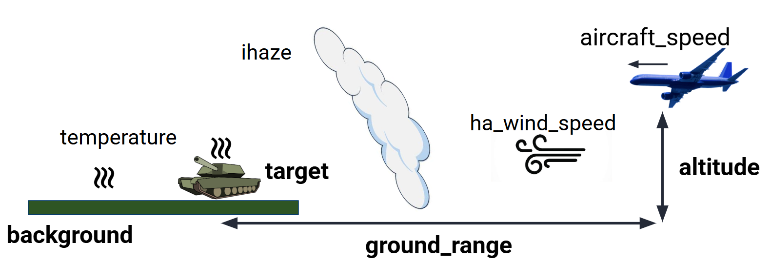
Figure 6: Depiction of scenario variables

More information is found at Scenario

Main Reference Image Variables

These variables contain information about the image target and the actual pixel values. An important function in ref_image is “estimate_capture_parameters” which can be used to estimate the camera sensor parameters used to capture the image given some scenario parameters. It is important to remember that the reference image is the ideal image, in that its quality will not be improved upon in the simulation but degraded or altered based on the parameters.

Key parameters include:

• img: the reference image data (array). This contains the pixel values of the image (required).

• gsd: the reference isotropic ground sampling distance (meters). This is the spatial sampling of the image, where the whole image is assumed to be a gsd x gsd square on the world surface (required).

• pix_values/refl_values: This is an optional parameter which associates pixel count values (i.e. 0 to 255) to scene reflectance values (i.e. 0 to 1), where pix_values and refl_values are equal-length arrays of the pixel values which correspond to reflectance values. This is important to set if you want to convert the pixel values to raw image values captured by the sensor, and it is important to take the non-linearities of the sensor encoding into account (default none, need to set both if using them).

Here is an example depiction of the pixel value to reflectance value mapping. The reason this is typically not linear is due to the gamma correction in the sensor, which mimics human perception rather than physical reflectance:

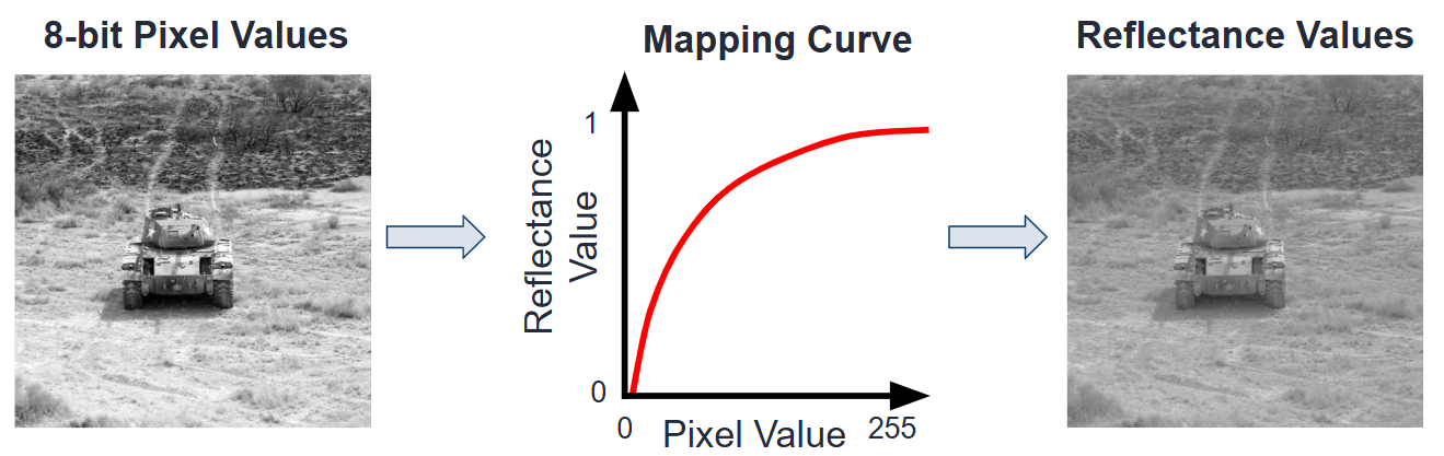
Figure 7: Depiction of pixel value to reflectance mapping function

Here is an example of GSD calculation. Note that this is given by the reference image but can also change based on sensor and scenario variables:

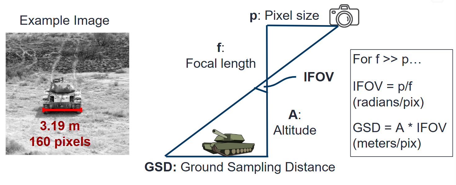
Figure 8: Depiction of GSD calculation based on sensor and scenario variables

More information is found at RefImage

Optical Transfer Function (OTF) Models

The main OTFs to consider are:

• circular_aperture_OTF/_with_defocus: Diffraction from optics and aperture (D , f)

• detector_OTF/_with_aggregation: Detector spatial integration effects, particularly important if fill factor is not 100% (p_x, p_y, w_x, w_y, f, n [pixels to aggregate])

• drift_OTF: Line-of-sight angular blur (da_x, da_y, int_time)

• filter_OTF: Custom filters (e.g., sharpening) (p_x, p_y, f)

• gaussian_OTF: Generic unmodeled Gaussian blur (Misc)

• jitter_OTF: Blur from high-frequency camera jitters (s_x, s_y)

• polychromatic_turbulence_OTF/turbluence_OTF: Atmospheric effects (opt_trans_wavelengths, altitude, ground_range, D, int_time, aircraft_speed, ha_wind_speed, cn_at_1m)

There are some more specialized OTFs contained in functional. These include cte_OTF (CCD charge transfer efficiency losses), diffusion_OTF (CCD minority carrier diffusion), tdi_OTF (time-delay-integration), wavefront_OTF (wavefront effects).